[Machine Learning] Regression & Classification

모두를 위한 딥러닝 (김성훈)

Colab_ML01-02
Colab_ML03
Colab_ML04
Colab_ML05
Colab_ML06

---

Regression

1. Linear Regression

하나의 독립변수 x에 의해 종속변수 y가 결정되는 선형 상관관계를 가진다.

1. data
2. Hypothesis: H(x) = Wx + b(W: weight, b: bias)
   cost가 가장 작은 가설을 선택
   cost function(loss function) = cost(W, b) = E( square(H(x) - y) )
3. goal: Minimize cost

 

Code

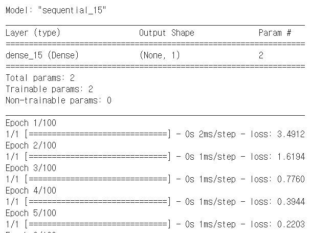
#Gradient Desendent Algorithm

import numpy as np
import tensorflow as tf

#1.dataSet 설정
x_train = [1, 2, 3, 4]
y_train = [2, 3, 4, 5]

#2.Model 구성
tf.model = tf.keras.Sequential()
    # units == output shape, input_dim == input shape
tf.model.add(tf.keras.layers.Dense(units=1, input_dim=1))

#3. Model 학습과정 설정
  # SGD == standard gradient descendent, lr == learning rate
sgd = tf.keras.optimizers.SGD(lr=0.1)
  # mse == mean_squared_error
tf.model.compile(loss='mse', optimizer=sgd)
  # prints summary of the model to the terminal
tf.model.summary()

#4. Model 학습
  # fit() executes training
  # 한 번의 epoch에서 모든 데이터를 한번에 넣을 수 X, 몇 번 나누어서 주는가를 iteration, 각 iteration마다 주는 데이터 사이즈를 batch size
tf.model.fit(x_train, y_train, epochs = 100)

#5. Model 사용하기
  # predict() returns predicted value
y_predict = tf.model.predict(np.array([5, 4, 3]))
print(y_predict)

 

Result

 

2. Multi-Variable Linear Regression

 Hypothesis and Cost

 Cost(W,b) = E( square(H(X)-Y) ) (X = [x], Y = [y] : training set

 이때 여러 H(x)중에서 cost를 최소값으로 가지는 가설을 선택한다.
 (그래프에서 W값이 x축, cost(W,b)가 y축에 위치)

 Gradient Descent Algorithm

 임의의 W점에서의 기울기를 통해, W값의 증가/감소가 결정된다. W를 움직여서 가장 기울기가 작은 곳(0에 수렴하는 W값)을 찾아가는 알고리즘.

기울기가 양수이면 다음 W값보다 작은 W의 왼쪽으로 이동하고, 기울기가 음수이면 다음 W값보다 큰 W의 오른쪽으로 이동한다.

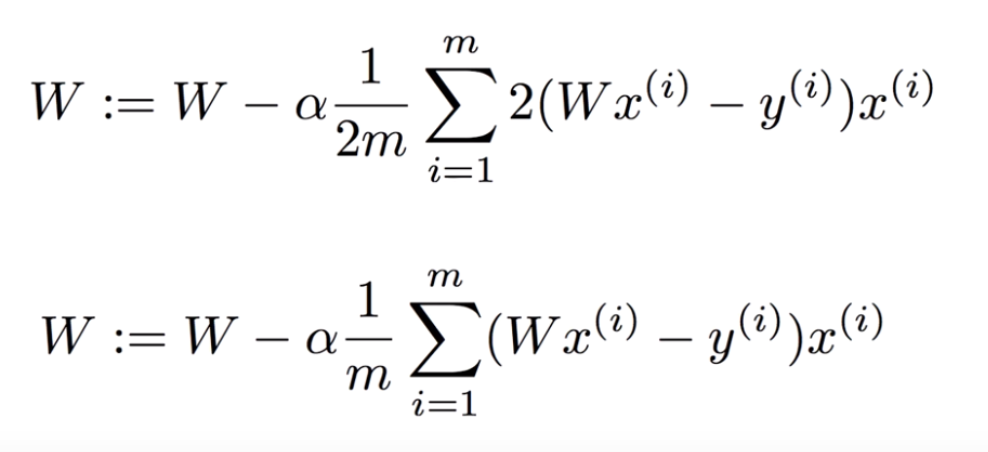
(W에서 빼고 있는 값은 LearningRate(a) * Cost'(: Cost의 기울기))
(계산에 큰 영향을 주지 않는 값들은 간략하게 처리)

Gradient Descent Algorithm으로 Linear Regression을 진행할 때,
Cost Function은 Convex Function(볼록 함수)

 

Code

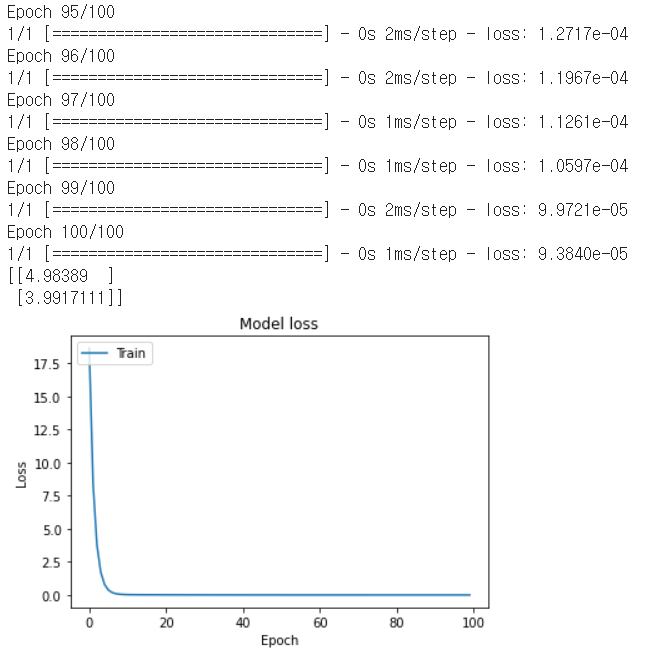
##Graph 그리기

import numpy as np
import tensorflow as tf
import matplotlib.pyplot as plt

#1.data set 설정
x_train = [1, 2, 3, 4]
y_train = [1, 2, 3, 4]

#2.Model 구성
tf.model = tf.keras.Sequential()
  # units == output shape, input_dim == input shape
tf.model.add(tf.keras.layers.Dense(units=1, input_dim=1))

#3. Model 학습과정 설정
  # SGD == standard gradient descendent, lr == learning rate
sgd = tf.keras.optimizers.SGD(lr=0.1)
  # mse == mean_squared_error, 1/m * sig (y'-y)^2
tf.model.compile(loss='mse', optimizer=sgd)
  # prints summary of the model to the terminal
tf.model.summary()

#4. Model 학습
  # fit() trains the model and returns history of train
history = tf.model.fit(x_train, y_train, epochs=100)

#6. Model 사용하기
  # predict() returns predicted value
y_predict = tf.model.predict(np.array([5, 4]))
print(y_predict)

  # Plot training & validation loss values
plt.plot(history.history['loss'])
plt.title('Model loss')
plt.ylabel('Loss')
plt.xlabel('Epoch')
plt.legend(['Train', 'Test'], loc='upper left')
plt.show()

 

Result

Multi-Variable Linear Regression

H(x) = Wx + b일 때는 변수가 한 개, 그러나 변수가 여러개인 상황에서는 Matrix의 곱셈을 이용하여 간략화할 수 있다. 따라서 행렬의 곱의 특징을 이해하는 것이 좋다.

X 행렬을 [a, b]라고 표현할 때, a는 instance의 개수, b는 variable의 개수를 의미한다.
W 행렬을 [b, c]라고 표현할 때, b는 variable의 개수, c는 가설의 X에 대한 Y값의 개수를 의미한다.(Linear에서, c = 1)
X 행렬과 Y 행렬의 곱이므로, H 행렬은 [a, c]라고 표현할 수 있다.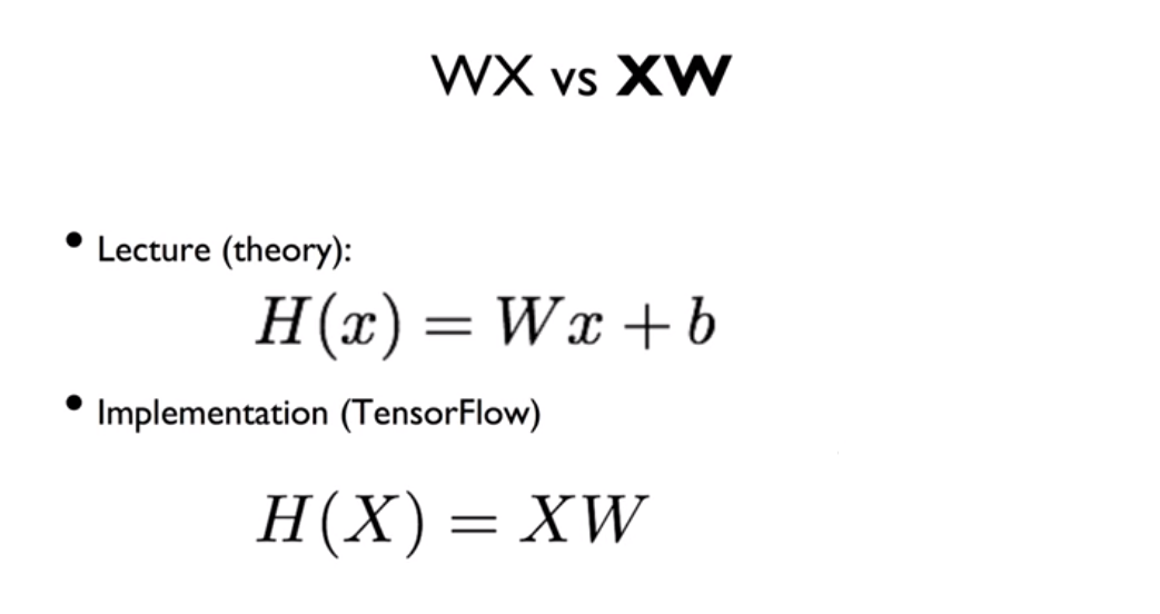

Matrix를 이용하면, W와 X의 순서가 바뀌는 것을 볼 수 있다. 따라서 H(X) = XW라고 표기하면, 행렬을 의미한다. 결론적으로 가설이랑 같은 의미를 가진다.

 

Code

##multi-variable regression

import tensorflow as tf
import numpy as np

#1.dataSet 설정
x_data = [[73., 80., 75.], [93., 88., 93.], [89., 91., 90.], [96., 98., 100.], [73., 66., 70.]]
y_data = [[152.], [185.], [180.], [196.], [142.]]

#2.Model 구성
tf.model = tf.keras.Sequential()
  # input_dim=3 gives multi-variable regression
tf.model.add(tf.keras.layers.Dense(units=1, input_dim=3))
  # linear activation is default
tf.model.add(tf.keras.layers.Activation('linear'))

#3. Model 학습과정 설정
tf.model.compile(loss='mse', optimizer=tf.keras.optimizers.SGD(lr=1e-5))

#4. Model 출력
tf.model.summary()

#5. Model 학습
history = tf.model.fit(x_data, y_data, epochs=100)

#6. Model 사용하기
y_predict = tf.model.predict(np.array([[72., 93., 90.],[60., 80., 80]]))
print(y_predict)

 

Result

Logistic Classification

3. Binary Classification

이산적인 결과를 가지며, 0과 1로의 encoding이 필요하다.

spam detection: spam or ham, facebook feed의 show or hide

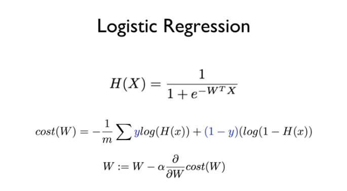
Hypothesis

-log(x) / -log(1-x)

sigmoid

 

Binary Classification은 0또는 1의 값을 가지기 때문에, 결과값이 0~1인 Sigmoid(S자형곡선)을 이용한 가설을 세울 수 있다. 위의 H(x)가 sigmoid 함수이며, logistic cost 함수라고도 한다. Cost 최소화는 Gradient Descent Optimizer를 사용하여 구현한다.

 

Cost

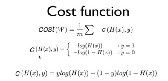
H(x) = 1H(x) = 0

Y = 1	0	INF
Y = 0	INF	0

 

Code

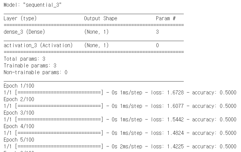
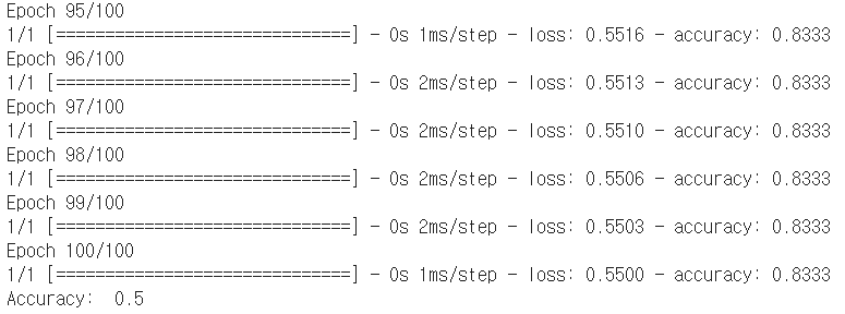
##binary classification

import tensorflow as tf

#1.dataSet 설정
x_data = [[1, 2],[2, 3],[3, 1],[4, 3],[5, 3],[6, 2]]
y_data = [[0], [0], [0], [1], [1], [1]]

#2.Model 구성
tf.model = tf.keras.Sequential()
tf.model.add(tf.keras.layers.Dense(units=1, input_dim=2))
tf.model.add(tf.keras.layers.Activation('sigmoid'))

#3. Model 학습과정 설정
tf.model.compile(loss='binary_crossentropy', optimizer=tf.keras.optimizers.SGD(lr=0.01), metrics=['accuracy'])

#4. Model 출력
tf.model.summary()

#5. Model 학습
history = tf.model.fit(x_data, y_data, epochs=100)#return np.array

#6. Model 사용하기
print("Accuracy: ", history.history['accuracy'][-1])

 

Result

4. Multinomial Classification

여러개의 선택지 중 하나를 선택하는 결과를 가진다.

위와 같이 세가지로 분류할 수 있다고 가정할 때, 3가지 Binary Classification을 진행하여 Multinomial Classification을 구현한다.

Hypothesis

세가지 가설을 행렬을 사용하여 간략화한다. binary의 경우에는 sigmoid 함수를 사용했지만, 여기서는 softmax 함수를 사용하여 예측값을 반환한다. softmax는 0부터 1사이의 값을 반환하며, 모든 출력값의 합이 1이다. One-Hot-Encoding은 배열 내 가장 큰 값을 1로, 나머지 값들은 0으로 반환한다. 결국 Y_data와 같은 결과를 가져온다.

 

Cost

Cross-Entropy
: 결론적으로 Logistic cost function과 결과가 같다. Cost 최소화는 Gradient Descent Optimizer를 사용한다.

 

Code

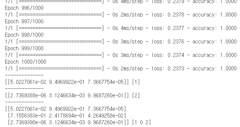
## multinominal classification
import tensorflow as tf
import numpy as np

#1.dataSet 설정
x_raw = [[1, 2, 1, 1],
         [2, 1, 3, 2],
         [3, 1, 3, 4],
         [4, 1, 5, 5],
         [1, 7, 5, 5],
         [1, 2, 5, 6],
         [1, 6, 6, 6],
         [1, 7, 7, 7]]
y_raw = [[0, 0, 1],
         [0, 0, 1],
         [0, 0, 1],
         [0, 1, 0],
         [0, 1, 0],
         [0, 1, 0],
         [1, 0, 0],
         [1, 0, 0]]
         #One Hot Encoding

x_data = np.array(x_raw, dtype=np.float32)
y_data = np.array(y_raw, dtype=np.float32)

nb_classes = 3

#2. Model 구성
tf.model = tf.keras.Sequential()
tf.model.add(tf.keras.layers.Dense(input_dim=4, units=nb_classes, use_bias=True))
  # use softmax activations: softmax = exp(logits) / reduce_sum(exp(logits), dim)
tf.model.add(tf.keras.layers.Activation('softmax'))

#3. Model 학습과정 설정
# use loss == categorical_crossentropy
tf.model.compile(loss='categorical_crossentropy', optimizer=tf.keras.optimizers.SGD(lr=0.1), metrics=['accuracy'])

#4. Model 출력
tf.model.summary()

#5. Model 학습
history = tf.model.fit(x_data, y_data, epochs=1000)

#6. Model 사용
print('--------------')
#출력 : One-hot encoding
# argmax : array에서 가장 큰값을 출력
a = tf.model.predict(np.array([[1, 11, 7, 9]]))
print(a, tf.keras.backend.eval(tf.argmax(a, axis=1)))

print('--------------')
# or use argmax embedded method, predict_classes
c = tf.model.predict(np.array([[1, 1, 0, 1]]))
c_onehot = tf.model.predict_classes(np.array([[1, 1, 0, 1]]))
print(c, c_onehot)

print('--------------')
all = tf.model.predict(np.array([[1, 11, 7, 9], [1, 3, 4, 3], [1, 1, 0, 1]]))
all_onehot = tf.model.predict_classes(np.array([[1, 11, 7, 9], [1, 3, 4, 3], [1, 1, 0, 1]]))
print(all, all_onehot)

 

Result